Tutorial 4: Accessing thermodynamic properties from sampling methods
In this tutorial you will learn how to calculate thermodynamic properties by using the Metropolis Monte-Carlo method or the Wang-Landau method. The application of both sampling methods will be demonstrated on the Pt/Cu(111) surface alloy.
The essential elements to carry out a sampling procedure are:
a cluster expansion (CE) model for the energy
spezification of the simulation cell
As CE model for the energy of the Pt/Cu(111) surface alloy, we use a CE model that can be downloaded here. You can also build the model yourself with the python script that is provided here. This can be initialized from the file “model-PtCu-2.pickle” with:
[1]:
from clusterx.model import Model
cemodelE = Model(filepath = "model-PtCu-2.pickle")
\(E_{\rm ads}\) predicted by this CE model is given in units of \(eV\) per subsitutional site, short \(eV/site\). How this CE model is obtained, is described in detail in tutorial_CE_Pt/Cu(111).
Now, we use the parent lattice for which the CE model is based on to create the simulation cell. Our simulation cell is an object of the class SuperCell, and can be initialized as:
[7]:
# Intialization of the SuperCell object being the simulation cell
from clusterx.super_cell import SuperCell
scell = SuperCell(cemodelE.get_plat(),[[4,0],[-2,4]])

# Display information of the SuperCell object
scell.get_sublattice_types(pretty_print=True)
sites_dict = scell.get_nsites_per_type()
for key in sites_dict.keys():
    print("Number of atoms in sublattice "+str(key)+":", sites_dict[key])

from clusterx.visualization import juview
juview(scell)
+--------------------------------------------------------------------+
|              The structure consists of 2 sublattices               |
+--------------------------------------------------------------------+
| Sublattice type |       Chemical symbols       |  Atomic numbers   |
+--------------------------------------------------------------------+
|        0        |            ['Cu']            |       [29]        |
|        1        |         ['Cu' 'Pt']          |      [29 78]      |
+--------------------------------------------------------------------+

Number of atoms in sublattice 0: 32
Number of atoms in sublattice 1: 16
As we see from the displayed information, the supercell consists of two sublattices, with indices 0 and 1. Both sublattices contain species “Cu”. In sublattice 0, they can not be substituted, while in sublattice 1 that contains all sites of one (111) surface, “Cu” can be substituted by “Pt”. This simulation cell has, in total, 16 substitutional surface sites:
[8]:
nsites = len(scell.get_substitutional_atoms())
print(nsites)
16
Metropolis Monte-Carlo sampling
In the following, we perform a Metropolis Monte-Carlo (MMC) sampling [N. Metropolis et. al., J. Chem. Phys. 21, 1087 (1953)] in the canonical ensemble, i.e. the volume of the simulation cell, the composition and the temperature remain unchanged. During such a sampling algorithm, a sequence of configurations is generated by modifying the configuration at each step by one or multiple swaps of two randomly-choosen species in the substitutional lattice(s). After a swap, the new proposed structure with energy \(E_1\) is accepted with the probability
\begin{equation*} P ( E_0 \rightarrow E_1) = \min \left[ \exp \left( - \frac{E_1-E_0}{k_{\rm B} T} \right) , 1 \right]. \end{equation*}
Here, \(E_0\) is the energy of the structure before the swap. This acceptance probability distribution depends on the Boltzmann probability distribution \(\exp \left( - \frac{E}{k_{\rm B} T} \right)\) at given temperature \(T\) and the Boltzmann constant \(k_{\rm B}\).
For canonical samplings in the surface alloy Pt/Cu(111), we choose a composition with 4 Pt atoms, e.g. a Cu\(_3\)Pt alloy in the surface layer. Now, we perform a MMC sampling at \(T=300\,\)K with:
[9]:
nsubs = {0:[4]}
kb = float(8.6173303*10**(-5)) # Boltzmann constant in eV/K
temp = 300 # Temperature in K

# Initialization of a MonteCarlo object
from clusterx.thermodynamics.monte_carlo import MonteCarlo
mc = MonteCarlo(cemodelE, \
                scell, \
                ensemble = "canonical", \
                nsubs = nsubs, \
                predict_swap = True)

# Execution of a Metropolis Monte-Carlo sampling
traj = mc.metropolis(no_of_sampling_steps = 1000, \
                     temperature = 800, \
                     boltzmann_constant = kb, \
                     scale_factor = [1/(1.0*nsites)])
In the first three lines, we define the number of Pt atoms in the substitutional lattice 1 by nsubs, \(k_{\rm B}\) and \(T\). Afterwards, we load the MonteCarlo class, and create an object of this class, called mc. The initialization of this object requires the CE model for the energy cemodelE, the simulation cell scell, and for a canonical sampling the composition defined by nsubs. As an option, you
can put predict_swap=True to speed up the sampling time (more details are given in the description of the class MonteCarlo). The object mc contains the main components to set up a sampling procedure, but does not perform a sampling by itself and is temperature independent.
Using the object mc, the MMC sampling can be executed with the method metropolis. As arguments, it needs the number of sampling steps no_of_sampling_step, \(T\) temperature, and \(k_{\rm B}\) boltzmann_constant. Here, the product \(k_{\rm B}T\) has to have the same units as the energies predicted by the CE model cemodelE. In our case, the units of \(E_{\rm ads}\) are \(eV/sites\), while the the product \(k_{\rm B}T\) is given in units of
\(eV\). To obtain the same units for \(k_{\rm B}T\), we make use of the optional argument scale_factor. scale_factor is a list of arbitrary length containing float numbers. The product of the floats is multiplied to \(k_{\rm B}T\). Thus, to get the units \(eV/sites\), we use scale_factor=[1/nsites].
The metropolis creates an object of the class MonteCarloTrajectory that stores all information of the trajectory generated from the MMC sampling. This object, named traj in the code above, is used to access this information after the MMC sampling. In the following, we show some examples how to obtained certain properties from the traj object (for more details please see the description of the class
MonteCarloTrajectory).
Below, we visualize e.g. the last structure visited in the MMC sampling:
[10]:
last_structure = traj.get_structure(-1)

#from clusterx.visualization import juview
juview(last_structure)
In the code shown below, we visualize the first three accepted structures in the sampling. For this, we first get the list of the accepted steps from the method get_sampling_step_nos. Then, in a for loop over the first three accepted steps of this list, Structure objects at these steps are created and stored. At the end the stored structures are visualized:
[12]:
steps_accepted = traj.get_sampling_step_nos()

first_three_accepted_structures = []
for step in steps_accepted[:3]:
        struc = traj.get_structure_at_step(step)
        first_three_accepted_structures.append(struc)

from clusterx.visualization import juview
#juview(last_structure)
juview(first_three_accepted_structures)
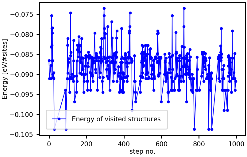
We can extract the energies of the accepted MMC steps with the method get_energies and plot them versus the sampling step number:
[13]:
energies_accepted = traj.get_energies()

%matplotlib inline
from clusterx.visualization import plot_property
plot_property(steps_accepted, energies_accepted, \
             prop_name = "Energy of visited structures", \
             xaxis_label = "step no.", yaxis_label = "Energy [eV/#sites]")
Next, we want to use the MMC method to study thermodynamic properties of the CuPt(111) surface alloy, as e.g. the isobaric specific heat \(C_p\).
\(C_p\) can be calculated from the MMC trajectory traj by the method calculate_average_property. As arguments, we define the property that we want to obtain with prop_name, in our case "C_p" for the specific heat, and the number of equilibration steps no_of_equilibration_steps that are discarded at the beginning of the sampling trajectory from the average, in our case we choose 100 equilibration steps.
[14]:
cp = traj.calculate_average_property(prop_name = "C_p", \
                                no_of_equilibration_steps = 100)
print("Specific heat for",temp,"K:", cp, "k_B/#sites")
Specific heat for 300 K: 0.10164517942599213 k_B/#sites
This single value does not say much. To study the temperature dependence of \(C_p\), we need to perform MMC samplings in a range of temperatures. This is done in the following piece of code (be aware that this sampling takes a few minutes):
[18]:
temp_list = []
cp_list = []

# Simulated annealing
for i,temp in enumerate(range(1400,0,-100)):
    if i == 0:
        init_structure = scell.gen_random(nsubs=nsubs)
    traj = mc.metropolis(no_of_sampling_steps = 1000, \
                         temperature = temp, \
                         boltzmann_constant = kb, \
                         scale_factor = [1/(1.0*nsites)], \
                         initial_decoration = init_structure.get_atomic_numbers())
    cp = traj.calculate_average_property(prop_name = "C_p", \
                         no_of_equilibration_steps = 200)

    print("Sampling at temperature ", temp, "K gives a specific heat of ", cp)
    temp_list.append(temp)
    cp_list.append(cp)
    init_structure = traj.get_structure(-1)
Sampling at temperature  1400 K gives a specific heat of  0.027353887641240214
Sampling at temperature  1300 K gives a specific heat of  0.03679968095733418
Sampling at temperature  1200 K gives a specific heat of  0.04247668684048657
Sampling at temperature  1100 K gives a specific heat of  0.05094406465862546
Sampling at temperature  1000 K gives a specific heat of  0.07468717007690714
Sampling at temperature  900 K gives a specific heat of  0.07628716451360108
Sampling at temperature  800 K gives a specific heat of  0.07990603709147324
Sampling at temperature  700 K gives a specific heat of  0.2039298875821653
Sampling at temperature  600 K gives a specific heat of  0.286716279255121
Sampling at temperature  500 K gives a specific heat of  0.33938655839719717
Sampling at temperature  400 K gives a specific heat of  0.0031864985531503843
Sampling at temperature  300 K gives a specific heat of  2.0697699861960484e-26
Sampling at temperature  200 K gives a specific heat of  3.9878459814233956e-26
Sampling at temperature  100 K gives a specific heat of  1.5951383925693582e-25
With the code above, a simulated annealing is performed. I.e. the for loop starts from a reasonable high temperature of \(T=1400\,\)K and gradually decreases \(T\) in steps of \(100\,\)K. For each temperature, an MMC sampling is performed and the \(C_p\) calculated. After each sampling, the last structure is stored as init_structure in order to use it as initial structure for the following MMC sampling. Here, for the first temperature, the MMC starts from a random
structure (initialized with the if case).
After the simulated annealing, we can visualize the lowest-energy structure visited at the last sampled temperature of \(T=100\,\)K with:
[19]:
juview(traj.get_lowest_energy_structure())
This structure is expected to show an ordered pattern. For the surface stoichiometry of Cu\(_3\)Pt, a \(p(2\times2)\) ordering is expected accoring to Ref. [F. R. Lucci et. al., J. Phys. Chem. C 118, 6, 3015 (2014)]. If your result is not showing this ordering, it can be due to an insufficent number of sampling steps.
The plot below shows the \(C_p\) versus temperature obtained from the simulated annealing. For a phase transition from an ordered ground state to disorderd state, \(C_p\) is expected to have a maximum at the transition temperature.
[20]:
plot_property(temp_list, cp_list, \
             prop_name = "Specific heat", \
             xaxis_label = "Temperature [K]", yaxis_label = r'C$_p$ [k$_B$/#sites]')
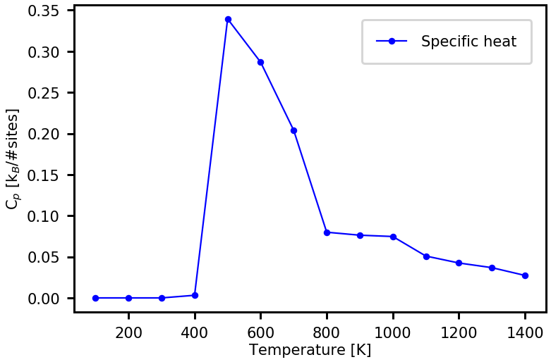
The parameters of the MMC samplings above are chosen to achieve fast samplings and give only rough estimates of actual properties of the system.
To determine a precise transition temperature of the order-disorder phase transition for the Pt/Cu(111) surface alloy, e.g. MMC samplings with larger sampling steps, in total, are required (see Excercises at the end). As another possibility to access thermodynamic properties, we present in the next section the Wang-Landau method.
Wang-Landau method
As an alternative to the MMC sampling, we present the Wang-Landau (WL) method [F. Wang and D. P. Landau, Phys. Rev. Lett. 86, 2050 (2001)]. Instead of performing temperature-dependent samplings, this methods obtains directly the temperature-independent configurational density of states \(g(E)\) from a single sampling procedure. Once the \(g(E)\) is known, thermodynamic properties at any desired temperature can directly be calculated.
Short introduction into the Wang-Landau method: In the WL sampling, the new structure proposed by a random swap of atoms with energy \(E_1\) and corresponding \(g(E_1)\) is accepted with the probability \begin{equation*} P(E_0 \rightarrow E_1) = \min \left[ 1, \frac{g(E_0)}{g(E_{1})} \right] \end{equation*} Here, \(E_0\) and \(g(E_0)\) are the energy and the corresponding configurational density of states of the previous structure. The acceptance probability is proportional to \(1/g(E)\). If the true \(g(E)\) is used in \(P(E_0 \rightarrow E_1)\), the sampling generates a flat histogram. Upon reversion, it means that if a sampling generates a flat histogram, the \(g(E)\) is close to the true \(g(E)\).
As a starting point for such a sampling, the complete energy space, that can be visited during a canonical sampling, is discretized into energy bins with predefined width \(\Delta E\). The \(g(E)\) of those bins is unknown, thus it is initially set to \(g(E)=1\) for all bins. Furthermore, the histogram of the sampling is initially set to \(H(E)=0\) (no visits). At each sampling step, independent of the acceptance or rejection of the new structure, \(g(E)\) and \(H(E)\) of the currently visited structure are updated with \(g(E)=g(E) \cdot f\) and \(H(E)=H(E)+1\). Here, \(f\) is the so-called modification factor, which is initially set to \(f=\exp(1)\). The sampling algorithm performs a nested loop consisting of an inner loop to generate a flat histogram for a given \(f\) and an outer loop that lowers \(f\) (usually by \(f \rightarrow \sqrt{f}\) in each iteration). The accuracy of the final \(g(E)\) depends on \(f\) and the flatness of the histogram. A histogram is considered as flat if the minimum of \(H(E)\) is larger than a fraction \(x\) of the mean value of \(H(E)\), i.e. \(\min H(E) > x \cdot \bar{H}(E)\). This fraction is usually \(x=0.5\) for the first iterations in the outer loop and is increased up to \(x=0.98\) in the last iterations (depends highly on the complexity of the system). Details about this method can be found in Ref. [F. Wang and D. P. Landau, Phys. Rev. Lett. 86, 2050 (2001)] and [D. P. Landau et. al., Am. J. Phys. 72, 1294 (2004)].
In the following, we use the class WangLandau to obtain the \(g(E)\) for surface alloy Pt/Cu(111) at the stoichiometry of Cu\(_3\)Pt, i.e. 4 Pt atoms in the 16 surface sites (be aware that the execution of the following code lines take a few minutes).
[22]:
nsubs={0:[4]}
emin = 12.7
emax = 13.9

# Initialization of a WangLandau object
from clusterx.thermodynamics.wang_landau import WangLandau
wl = WangLandau(cemodelE,
                scell,
                ensemble = "canonical",
                nsubs = nsubs,
                predict_swap = True,
                error_reset=None)

import numpy as np
# Execution of the Wang-Landau sampling
cdos = wl.wang_landau_sampling(energy_range = [emin, emax],
                               energy_bin_width = 0.025,
                               f_range = [np.exp(1), np.exp(1e-2)],
                               flatness_conditions=[
                                    [0.8,np.exp(1e-1)],
                                    [0.90,np.exp(1e-3)],
                                    [0.95,np.exp(1e-5)]
                                ],
                               serialize = True,
                               serialize_during_sampling = True,
                               filename = 'cdos.json')
In the first line, we define the number of Pt atoms in the substitutional lattice 1 by nsubs. Afterwards, we initialize an object wl of the WangLandau class with the same arguments used to initialize a MonteCarlo object, i.e. the CE model for the energy cemodelE, the simulation cell scell, and the composition defined by nsubs (optional predict_swap=True).
Using the object wl, the WL sampling can be executed with the method wang_landau_sampling. It needs the following arguments: - the energy range energy_range defined by a list containing the minimum energy (first entry in list) and the maximum energy (secondt entry), that covers the complete energy space visited during the canonical sampling, - the discretization of the energy range \(\Delta E\) energy_bin_width, - the range of the modification factor f_range defined by a
list contining the initial \(f\) (first entry in list) and a threshold for the final \(f\) (second entry) (if the next proposed \(f\) is below this threshold, the WL sampling stops), - and optional arguments as serialize to serialize the cdos object after the sampling, serialize_during_sampling to serialize the cdos object after every iteration of the outer loop during the sampling, and filename to set the name of the file in which the cdos is stored. (more
details are given in the description of the class WangLandau)
The returned object cdos is an object of the class ConfigurationalDensityOfStates and contains all information about the \(g(E)\) obained at each iteration of the outer loop in the WL algorithm. If the option serialize_during_sampling is set to True, the information can be accessed even during the WL sampling. This is done by reading the ConfigurationalDensityOfStates object from file
(see code lines below).
In the following, we show some examples how to obtained thermodynamic properties from the wl object (for more details please see the description of the class ConfigurationalDensityOfStates).
In the first three lines of the code below, we define the temperatures, for which we want to calculate the thermodynamic properties, the Boltzmann constant \(k_{\rm B}\) and also a scale factor scale_factor used to have the product \(k_{\rm B}T\) in the same units as the CE model of the energy (here \(E_{\rm ads}\) is given in units of \(eV/sites\)). Next, the ConfigurationalDensityOfStates object is read from the file cdos.json. This object, called cdos_read, is
used to access \(g(E)\) and to visualize \(ln(g(E))\) with plot_property. Afterwards, the specific heat \(C_p\) and the internal energy \(U\) are calculated and visualized too. You will recognize that the execution of the following code line will be fast.
[23]:
temps = range(150,1500,10)
scale_factor = [1/(1.0*nsites)]

# Reading of configurational density of states from file, e.g. cdos2.json as produced before
from clusterx.thermodynamics.wang_landau import ConfigurationalDensityOfStates
cdos_read = ConfigurationalDensityOfStates(filename = 'cdos.json', read = True)

e, lng = cdos_read.get_cdos(ln = True, normalization = True)
from clusterx.visualization import plot_property
plot_property(e,lng, xaxis_label = "E [eV/sites]", yaxis_label = "ln(g(E))", prop_name="lng")

cp = cdos_read.calculate_thermodynamic_property( temps, prop_name = "C_p")
plot_property(temps,cp, xaxis_label = "Temperature [K]", yaxis_label = "Specific heat [k_B/#sites]", prop_name = "C_p")

u = cdos_read.calculate_thermodynamic_property( temps, prop_name = "U")
plot_property(temps,u, xaxis_label = "Temperature [K]", yaxis_label = "Internal energy [eV/#sites]", prop_name = "U")
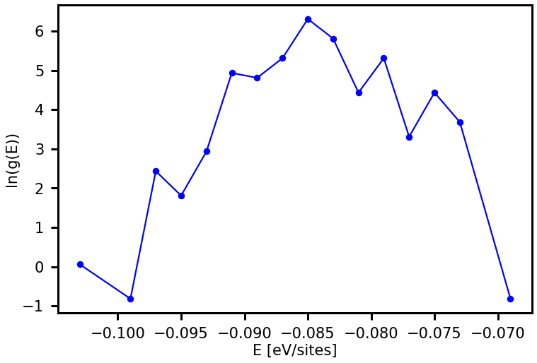
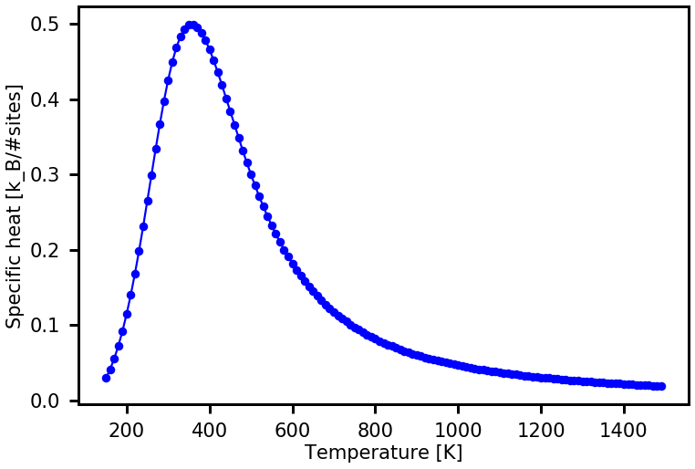
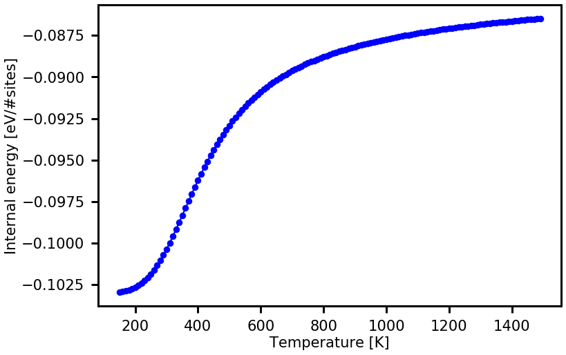
The \(g(E)\) and the resulting thermodynamic property do not look converged yet. This is due to the fact that we choose a fairly large final modification factor of \(f=\exp (0.1)\). The WL sampling usually yields converged results if the final \(f\) is \(\exp(0.0001)\) or even much lower (this requires a larger sampling time).
Excercise 6: Metropolis Monte-Carlo sampling
Perform a simulated annealing with a larger number of sampling steps for the MMC sampling at each temperature than it was used in the example above.
Increase the simulation cell size, e.g. a Pt/Cu(111) surface alloy with \(64\) surface sites, and repeat the simulated annealing or a single MMC sampling. How does it affect the transition temperature?
Be aware that the execution of those samplings can take up to a few days (depending on the choice of parameters).
Excercise 7: Wang-Landau sampling
Choose a lower threshold for the final modification factor for the WL sampling than it was used in the example above.
In the method
wang_landau_samplingof theWangLandauobject above, we do not set explizitly the flatness condition. Look at the documentation of the class WangLandau to find out which flatness conditions are used as default. The flatness condition for each iterater in the outer loop can be also read from the serialized file of theConfigurationalDensityOfStatesobject. Try to change the modification factors.Increase the simulation cell size. Is the peak of the \(C_p\) changing?
Also, here, be aware that the execution of those samplings can take up to a few days (depending on the choice of parameters).
[ ]: