Tutorial 3: Building and optimizing a CE model

In this tutorial, you will learn how to build a cluster expansion model for a complex surface system.

The optimal model

Once a training data set and a pool of clusters are available, the next task is to compute a property of interest, and build a CE model for that property.

With this model, we will be able to efficiently predict property values for arbitrary structures.

This task requires finding the set of clusters that best describes the relevant interactions present in the system. Various optimality criteria can be used.

Here we will focus on obtaining models which are optimal in the sense of providing the best possible predictions for new data, i.e., data not yet included in the training set.

For this purpose, the quality of the predictions of a CE model can be estimated by cross validation (CV), which you will learn to calculate and interpret in this section.

Here, we will use the surface system with oxygen adsorption and Na substitution, which was used in Tutorial 1, to build a cluster expansion model. We start by generating the needed elements for the task, namely a training data set and a pool of clusters.

[ ]:

%matplotlib inline
from ase.build import fcc111, add_adsorbate # ASE's utilities to build the surface
from clusterx.parent_lattice import ParentLattice
from clusterx.structures_set import StructuresSet
from clusterx.visualization import juview
from clusterx.super_cell import SuperCell
from random import randint
import numpy as np

# seed random generators for reproducibility
import random
np.random.seed(10)
random.seed(10)
############################################

# Build a 3-layer Al slab with vacancy in on-top configuration
pri = fcc111('Al', size=(1,1,3))
add_adsorbate(pri,'X',1.7,'ontop')
pri.center(vacuum=10.0, axis=2)

# Build the parent lattice and a 4x4 supercell
platt = ParentLattice(pri, site_symbols=[['Al'],['Al'],['Al','Na'],['X','O']])
platt.print_sublattice_types() # Print info regarding the ParentLattice object
scell = SuperCell(platt,[4,4])

# Collect 60 random structures in a StructuresSet object
sset = StructuresSet(platt)
nstruc = 60

for i in range(nstruc):
    concentration = {0:[randint(0,4*4)],
                     1:[randint(0,4*4)]} # Pick a random concentration of "Na" substitutions and "O" adsorbants

    sset.add_structure(scell.gen_random(concentration)) # Generate and add a random structure to the StructuresSet

print("\nRandom structures (first 3):")
sset.serialize("sset.json") # Write JSON db file for visualization with ASE's GUI.
juview(sset,n=3) # Plot the first 3 created random structrues

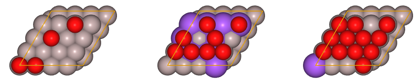
We have just created 60 random structures at several concentrations.

For this tutorial, we will build a model that predicts total energies. For that purpose, we need first to calculate the total energies of the training set ab initio.

In order to save time in this tutorial, we will not compute the energies with an ab initio code like `exciting <https://www.exciting-code.org>`__, but instead we will use the Effective Medium Theory calculator from ASE. The energies provided by this ab initio calculator are not very realistic, but serve the purpose to test and aquire basic training on the CE methodology.

[ ]:

from clusterx.calculators.emt import EMT2 # Load the CELLs wrapper of the EMT calculator from ASE
from clusterx.visualization import plot_property_vs_concentration

sset.set_calculator(EMT2())
sset.calculate_property("total_energy_emt") # Calculate energies with Effective Medium Theory calculator of ASE

In the next cell, we will create two structures free of oxygen adsorbants:

pristine, non-substituted (energy \(E_0\)) and
fully substituted one (Al->Na) (energy \(E_1\)).

and use the energies \(E_0\) and \(E_1\) as references for plotting the total energy: We will not plot directly the total energy E, but a partial energy of mixing

\[e=E - [ E_0*(1-x)+E_1*x ]\]

that is, the difference between the total energy and a linear interpolation between the pristine and fully substituted surface. Here \(E\) is the EMT energy of the structure and \(x\) the Na concentration.

[ ]:

refs = StructuresSet(platt)
refs.add_structure(scell.gen_random({0:[0],1:[0]})) # Pristine
refs.add_structure(scell.gen_random({0:[0],1:[16]})) # Full Na substitution
refs.set_calculator(EMT2())
refs.calculate_property("total_energy_emt_refs")
ref_en = refs.get_property_values("total_energy_emt_refs")

plot_data = plot_property_vs_concentration(
    sset,
    site_type=1,
    property_name="total_energy_emt",
    yaxis_label='Total energy',
    refs=ref_en
)

The information in this figure comprises the training set. The \(x\) axis indicates the concentration of Na on the top-most layer. For a given Na concentration, several points in the plot correspond to different structures of the training set having different arrangements of Na and O atoms, and/or different concentration of O atoms. The units of energy are arbitrary.

The next step is to create a pool of cluters:

[ ]:

r=3.5
from clusterx.clusters.clusters_pool import ClustersPool
cpool = ClustersPool(platt, npoints=[1,2,3,4], radii=[0,r,r,r])
print(len(cpool)," clusters were generated.")

[ ]:

cpool.serialize(db_name="cpool.json")
juview(cpool.get_cpool_atoms(),n=6)

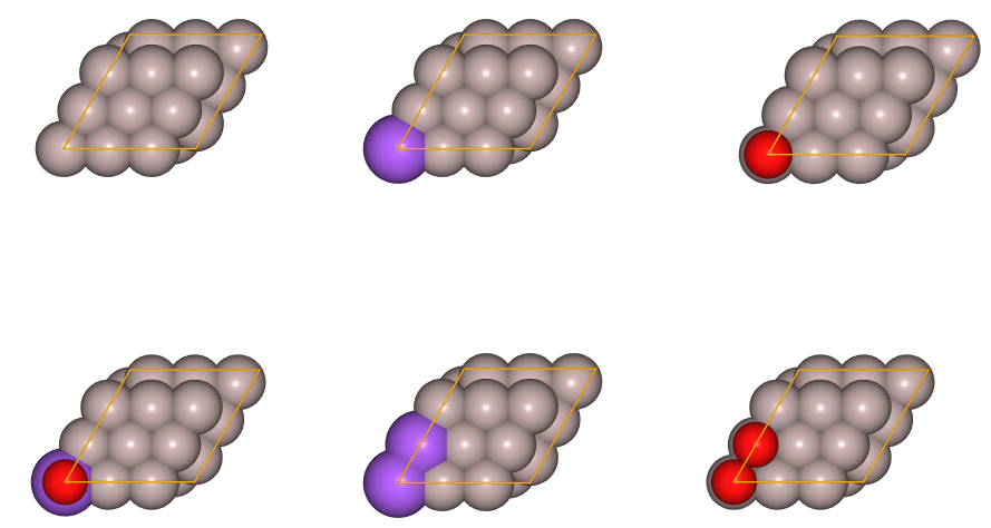
Above, only a few of the training structures and generated clusters are displayed. If you would like to visualize them all, use the ASE’s gui interface as explained in Tutorial 2.

Now that we have the basic elements, i.e., the training set sset and the pool of clusters cpool, we can proceed to build different CE models and to analyze the corresponding predictions.

This is achieved by using the ModelBuilder class of CELL.

The input parameters of this class determine how to perform two essential tasks, namely:

the selection of relevant clusters, and
the fitting procedure

For the first task, “selection of relevant clusters”, the important parameters are selector_type and selector_opts. We will use two different selectors: subsets_cv, which uses a cross validation strategy on cluster subsets of increasing size, and lasso, which uses compressed sensing techniques to obtain sparse models.

For the second task, i.e. “the fitting procedure”, the relevant parameters are estimator_type and estimator_opts. For the example in this tutorial, we will fit our models with the LinearRegression estimator of sci-kit learn. Note that all the scikit-learn estimators are available in CELL through the EstimatorFactory class.

The ModelBuilder encapsulates several complex tasks embodied in classes like ClustersSelector, EstimatorFactory, CorrelationsCalculator, etc. which can be used separately in more advanced applications of CELL.

Now, run the following listing and analize the reported results:

[ ]:

from clusterx.model import ModelBuilder

mb = ModelBuilder(
    selector_type="subsets_cv",
    selector_opts={'clusters_sets':'size'},
    estimator_type="skl_LinearRegression",
    estimator_opts={}
)

cemodel1 = mb.build(sset, cpool, "total_energy_emt") #Build CE model using the training data set
cpool_opt1 = mb.get_opt_cpool()

cemodel1.report_errors(sset)
cpool_opt1.print_info(ecis=cemodel1.get_ecis())
cpool_opt1.write_clusters_db(db_name="cpool_opt.json")

Two tables are printed.

The first Table contains a detailed report of prediction errors for the optimal model found by ModelBuilder.

The column Fit indicates the errors of the fit to the training data. The column CV reports the estimate of the test error by cross validation.

Different metrics are used: the row RMSE indicates the root-mean-squared-error, MAE the mean absolute error, and MaxAE the maximum absolute error. Observe that in general the errors from CV are slightly larger than for the fit. Why is this so?

The second table shows information on the optimal pool of clusters and the corresponding effective cluster interactions (ECI). Note that for clusters with increasing number of points and radius, the interactions get smaller. Can you think of a reason for this behavior?

In the next listing we will generate three figures that are very informative:

The first of them shows how the optimality criterium based on CV works: For increasing numbers of clusters, the error of the fit (label “training-RMSE”) decreases monotonously. In contrast, the CV score (label “cv-RMSE”) has a minimum, which represents the crossover from models showing underfitting, i.e. poor fitting due to having few parameters, and models presenting overfitting, i.e. models with too many parameters (i.e. clusters), which are prone to fit noise. The red circle in this figure indicates the optimal model found.

The second plot shows, for every structure in the training set, the calculated energy versus the predicted energy. Since all the points lie in the solid stright line, this means that the predictions are good.

The third plot shows the calculated, predicted, and cross validated predictions as a function of Na concentration. As you can see, the predictions are quite accurate except for a few data points. Also, the predicted values are consistently better than the cross-validated predictions, as expected.

[ ]:

from clusterx.visualization import plot_optimization_vs_number_of_clusters
from clusterx.visualization import plot_predictions_vs_target

plot_optimization_vs_number_of_clusters(mb.get_selector())

plot_predictions_vs_target(sset,cemodel1,"total_energy_emt")

plot_data=plot_property_vs_concentration(
    sset,
    site_type=1,
    property_name="total_energy_emt",
    cemodel=cemodel1,
    yaxis_label='Total energy',
    refs=ref_en
)

Next, we will experiment with a different optimization procedure by changing the clusters_sets parameter from "size" to "size+combinations". For this, we need to specify two additional parameters, nclmax and set0.

In this case, the subsets for the CV procedure will be formed by the union of two sets: one of them considers all possible subsets of clusters up to nclmax, while the other is a fixed pool specified by set0.

set0 = [integer, float] is a list containing an integer and a float. They indicate, respectively, the maximum number of points and the maximum radius of any cluster in the fixed pool.

For instance, for set0 = [1,0], the fixed pool will contain a one point cluster of radius 0 (that’s obviously the maximum radius a 1-point cluster may have…).

Below a minimal example of this is given:

[ ]:

mb = ModelBuilder(
    selector_type="subsets_cv",
    selector_opts={
        'clusters_sets':'size+combinations',
        'nclmax':1,
        'set0':[1,0]},
    estimator_type="skl_LinearRegression",
    estimator_opts={}
)

cemodel2 = mb.build(sset, cpool, "total_energy_emt") #Build CE model using the training data set
cpool_opt2 = mb.get_opt_cpool()

cemodel2.report_errors(sset)
cpool_opt2.print_info(ecis=cemodel2.get_ecis())
cpool_opt2.write_clusters_db(db_name="cpool_opt2.json")

[ ]:

plot_optimization_vs_number_of_clusters(mb.get_selector())

plot_predictions_vs_target(sset,cemodel2,"total_energy_emt")

_=plot_property_vs_concentration(
    sset,
    site_type=1,
    property_name="total_energy_emt",
    cemodel=cemodel2,
    yaxis_label='Total energy',
    refs=ref_en
)

As you can see, the selection of small values for the parameters nclmax and set0 leads to poor quality of the predictions above.

Below, larger values are set for these parameters. The combinatorial search takes more time now, but the quality of the model improves considerably:

[ ]:

mb = ModelBuilder(
    selector_type="linreg",
    selector_opts={
        'clusters_sets':'size+combinations',
        'nclmax':3,
        'set0':[2,3.5]},
    estimator_type="skl_LinearRegression",
    estimator_opts={})

cemodel3 = mb.build(sset, cpool, "total_energy_emt") #Build CE model using the training data set
cpool_opt3 = mb.get_opt_cpool()

cemodel3.report_errors(sset)
cpool_opt3.print_info(ecis=cemodel3.get_ecis())
cpool_opt3.write_clusters_db(db_name="cpool_opt3.json")

[ ]:

plot_optimization_vs_number_of_clusters(mb.get_selector())

plot_predictions_vs_target(sset,cemodel3,"total_energy_emt")

_=plot_property_vs_concentration(
    sset,
    site_type=1,
    property_name="total_energy_emt",
    yaxis_label='Total energy',
    cemodel=cemodel3,
    refs=ref_en
)

In the next example, we will perform cluster selection with LASSO (Least Absolute Shrinkage and Selection Operator), using cross validation for selecting the sparsity hyper-parameter.

To this end, we change the first argument from "subsets_cv" to "lasso", and we indicate the sparsity range (sparsity_max and sparsity_min) for the hyper-parameter determination through cross-validation.

[ ]:

mb = ModelBuilder(
    selector_type="lasso",
    selector_opts={
        'sparsity_max': 0.1,
        'sparsity_min': 0.001},
    estimator_type="skl_LinearRegression",
    estimator_opts={}
)

cemodel4 = mb.build(sset, cpool, "total_energy_emt") #Build CE model using the training data set
cpool_opt4 = mb.get_opt_cpool()

cemodel4.report_errors(sset)
cpool_opt4.print_info(ecis=cemodel4.get_ecis())
cpool_opt4.write_clusters_db(db_name="cpool_opt4.json")

[ ]:

plot_optimization_vs_number_of_clusters(mb.get_selector())

plot_predictions_vs_target(sset,cemodel4,"total_energy_emt")

_=plot_property_vs_concentration(
    sset,
    site_type=1,
    property_name="total_energy_emt",
    yaxis_label='Total energy',
    cemodel=cemodel4,
    refs=ref_en
)

In order to see if the selected sparsity range contains the optimal sparsity, it is very informative to plot the cross-validation procedure for the hyperparameter. This is done with the plot_optimization_vs_sparsity function of the visualization module:

[ ]:

from clusterx.visualization import plot_optimization_vs_sparsity
plot_optimization_vs_sparsity(mb.get_selector())

Excercise 5

Perform a model optimization for the square Si-Ge binary lattice of Tutorial 2. Use the different strategies explained in this tutorial, i.e.: "subsets_cv" with "size" and "size+combinations" and "lasso". Interpret the results.

[ ]: