Tutorial 2: Clusters and cluster correlations¶

Building a pool of clusters¶

In Tutorial 1 you learned how to build parent lattices and structure sets. The next task is to create a pool of clusters

A clusters pool can be used to define the basis set for the expansion of configuration-dependent properties in terms of cluster functions \(\Gamma_\alpha(\sigma)\), such that a given configuration-dependent property \(P(\sigma)\) can be expanded in term of them

Although this basis is infinite (equal in number to all symetrically distinct atomic configurations of the substituent species), in practical applications one must cut off the basis. Here up to a number of clusters \(N_c\).

In order to fix ideas, we will start with a very simple model (corresponding to the solution of Excercise 1 of Tutorial 1) of a binary two-dimensional square lattice.

Afterwards, you will tackle the more complicated fcc(111) Al surface system of Tutorial 1, by solving Excercise 4 of this tutorial.

To start, we must define the parent lattice:

[ ]:

from ase import Atoms
from clusterx.parent_lattice import ParentLattice
from clusterx.visualization import juview
import numpy as np

a=4.0
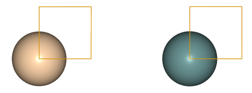
pri = Atoms(positions=[[0,0,0]],cell=[[a,0,0],[0,a,0],[0,0,2*a]],pbc=(1,1,0)) # Atoms object. Only positions and cell are set

plat = ParentLattice(pri,symbols=[['Si','Ge']]) # ParentLattice object with assignement of species to position "[[0,0,0]]"

juview(plat)

Now, we will create all possible clusters of up to four points and radius up to \(\sqrt{2}\,a\). This is done with the following lines of code:

[ ]:

from clusterx.clusters.clusters_pool import ClustersPool

r = 1.42 # This is large enough to include all clusters up to sqrt(2)*a
cpool = ClustersPool(plat, npoints=[1,2,3,4], radii=[0,a*r,a*r,a*r])

In the first line, we load the ClustersPool class. Then, we create an object of this class, and call it cpool.

To initialize it, we use the parameters npoints and radii. npoints indicates the number of points of the clusters in the pool, and the parameter radii indicates the maximum radius corresponding to each of the number of points indicated in npoints.

In this way, we have created a clusters pool containing the 1-point clusters (in this case there will be only one of this kind), and all the 2-, 3-, and 4-point clusters up to radius \(1.42\times a\).

The number of clusters just created is:

[ ]:

print("Number of clusters: ", len(cpool))

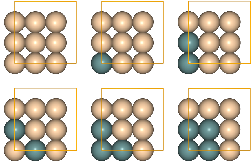
Now, we have at least two ways of visualizing the pool of clusters: i) we can plot all of them on this notebook with juview (or only a few, by using the parameter n of juview):

[ ]:

juview(cpool)

or ii) by using the graphical user interface (gui) of ASE on a terminal. To use this second option, which is the recommended way to proceed when the clusters pool is large, first serialize the database with

[ ]:

cpool.serialize()

The execution of this line will create a file called cpool.json in the same folder where this tutorial is run. This file has the proper format to be visualized with ASE’s gui. Now, open a terminal and execute $>ase gui cpool.json (the $> denotes the bash command prompt). A number of windows will open. The relevant ones for the visualization of the clusters are shown in the screen capture below:

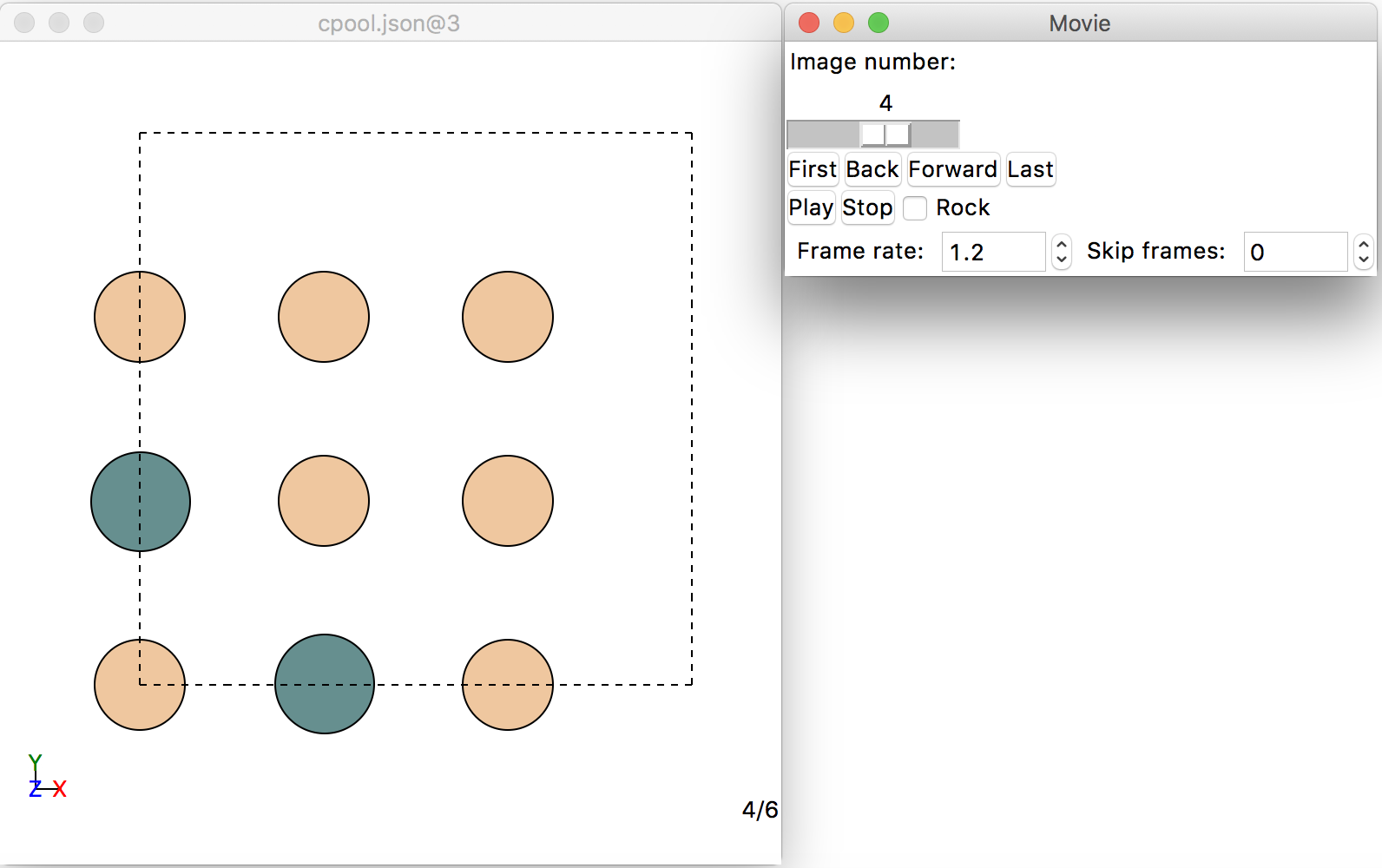
You can visualize all the clusters by clicking on the “Back” and “Forward” buttons of the “Movie” window on the right. Let’s see how this works for a larger clusters pool:

[ ]:

r = 2.5

cpool = ClustersPool(plat, npoints=[1,2,3,4,5], radii=[0,a*r,a*r,a*r,a*r])
cpool.serialize()

print(len(cpool), " clusters were created.")

So, now 33 clusters have been created. Let’s visualize clusters 7 to 9

[ ]:

juview(cpool,[7,10])

Now, as an excercise, create a clusters pool database and visualize these 33 clusters with ASE’s gui as explained above.

[ ]:

# You can write and execute your code here.

Cluster orbits¶

The clusters obtained above are all symmetrically inequivalent. Moreover, each of them is a representative of an (infinite) set of symmetrically equivalent clusters. Every of these sets is called a cluster orbit.

We can calculate a cluster orbit for a supercell and visualize it with either juview or ASE’s gui. Let’s do so for one cluster of the clusters pool cpool:

[ ]:

# Obtain the orbit for cluster number 7
cluster_orbit = cpool.get_cluster_orbit(cluster_index = 7)
cluster_multiplicity = cluster_orbit.get_reduced_multiplicity()

print("There are ",len(cluster_orbit),"symmetrically equivalent representations of the cluster in the supercell.")
print("The cluster multiplicity is ",cluster_multiplicity,".")

The cluster multiplicity is the number of symetrically equivalent realizations of the cluster, under the symmetry operations of the parent cell, without counting the internal translations of the parent cell inside the supercell. Or, equivalently, the number of symetrically equivalent clusters per unit cell.

Now, we create a clusters database containing the cluster orbit:

[ ]:

cluster_orbit.serialize(json_db_filepath="cluster_orbit.json")

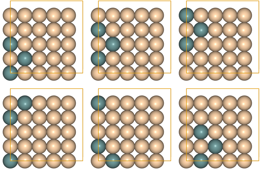
After this, you may visualize the cluster orbit by executing the command $>ase gui cluster_orbit.json in a terminal. Alternatively (without the need of executing the line above), you can use juview, as exemplified here by plotting the first 6 clusters of the orbit:

[ ]:

juview(cluster_orbit,n=6)

Cluster correlations¶

In this section we will illustrate the calculation of the cluster correlations for the simple binary case studied here. To simplify the analysis, we will use a (non-orthogonal) basis-set consisting of the following site cluster functions:

\begin{equation*} \gamma_0(\sigma_i) = 1\\ \gamma_1(\sigma_i) = \sigma_i. \end{equation*}

Here \(\sigma_i\) is the site occupation variable for the crystal site \(i\). \(\sigma_i=1\) if the crystal site \(i\) is occupied with the substitutional species (Ge in this example), or the value \(\sigma_i=0\) otherwise (Si in this example).

The first function, \(\gamma_0\), is the constant function, while the second, \(\gamma_1\), is an indicator function, taking the value 1 if the crystal site is occupied by Ge, and 0 if it is occupied by Si. Thus, it indicates if the site has been substituted.

Using this basis, one can define a basis set of cluster functions \(\Gamma_\alpha(\sigma_{s})\), with \(\sigma_{s}=(\sigma_{s1},\sigma_{s2},...,\sigma_{sN})\) a vector representing the configuration of the structure \(s\), and \(\alpha=\{\alpha_1,\alpha_2,...,\alpha_N\}\) a set of site cluster function indices representing a cluster (\(\alpha_i=0,1\) for \(\gamma_0\) and \(\gamma_1\), respectively):

\begin{equation*} \Gamma_\alpha(\sigma_{s})=\prod_{i=1}^N\gamma_{\alpha_i}(\sigma_{si}) \end{equation*}

since \(\gamma_0=1\), independently of \(\sigma\), the product in the equation above can be restricted to the cluster of lattice sites \(i\) for which \(\alpha_i=1\):

\begin{equation*} \Gamma_\alpha(\sigma_{s})=\prod_{i}^{\alpha_i=1}\gamma_1(\sigma_{si})=\prod_{i}^{\alpha_i=1}\sigma_{si} \end{equation*}

According to this definition, \(\Gamma_\alpha(\sigma_{s})=1\) if the substitutional pattern represented by cluster \(\alpha\) is present in structure \(s\), and \(\Gamma_\alpha(\sigma_{s})=0\) otherwise.

Using the symmetries of the pristine crystal, the cluster correlations \(X_{s\alpha}\) are obtained from the orbit-averaged cluster-functions:

\begin{equation*} X_{s\alpha}=\frac{1}{M_\alpha}\sum_{\beta\in{\cal O}({\alpha})}{\Gamma_\beta(\sigma_{s})} = \frac{M_{\alpha\in s}}{M_\alpha} \end{equation*}

Here, \({\cal O}({\alpha})\) is the set of all clusters in the orbit of \(\alpha\), \(M_{\alpha\in s}\) the number of clusters from \({\cal O}({\alpha})\) which are present in structure \(s\), and \(M_\alpha\) is the total number of clusters in \({\cal O}({\alpha})\).

In simpler terms we can say that the correlation \(X_{s\alpha}\) represents the concentration of the cluster (substitutional pattern) \(\alpha\) in structure \(s\).

Note that this interpretation is only valid in the case of binary alloys for the basis used in this example. The more general definitions of basis sets for multicomposition/multilattice alloys in CELL do not admit this interpretation.

Let’s now calculate the cluster correlations for the same small pool of 6 clusters obtained at the start of this tutorial:

[ ]:

r = 1.42
cpool = ClustersPool(plat, npoints=[1,2,3,4], radii=[0,a*r,a*r,a*r])
juview(cpool)

To accomplish this task, we must first create a CorrelationsCalculator object:

[ ]:

from clusterx.correlations import CorrelationsCalculator

corrcal = CorrelationsCalculator("indicator-binary", plat, cpool)

By using the paramenter "indicator-binary", the correlations will be computed using the basis set explained above.

Let’s now create a random structure and then obtain the cluster correlations for this structure:

[ ]:

from clusterx.super_cell import SuperCell

# seed random generators for reproducibility
import random
np.random.seed(0)
random.seed(0)
############################################

scell = SuperCell(plat,[4,4]) # Create a 4x4 supercell
structure = scell.gen_random({0:[3]}) # Random structure with 3 substitutional atoms
juview(structure.get_atoms())

Now, we calculate the correlations for this structure and display some relevant information, namely,

1. the cluster index \(\alpha\),

2. the length of the orbit for the cluster in the supercell (\(M_\alpha\)), and

3. the correlation of cluster \(\alpha\) to structure \(s\) (\(X_{s\alpha}\)).

[ ]:

corrs = corrcal.get_cluster_correlations(structure) # Compute correlations for structure
orbl = corrcal.get_orbit_lengths(structure) # Get orbit lengths in structure M_\alpha

print(f'{"Cluster index":<19s}|{"Orbit length":<19s}|{"Correlation":<19s}')
for i in range(len(cpool)):
    print(f'{i:<19d}|{orbl[i]:<19d}|{corrs[i]:<19.5f}')

Excercise 3¶

1. Using the figures of the clusters, the figure of the random structure generated above, and the orbit lengths, calculate by hand the correlations for the random structure and verify that they are equal to what is returned by the get_cluster_correlations() method.

2. Generate a new random structure with a different concentration, recalculate the correlations, and repeat item a).

3. To which familiar quantity can you relate the correlation for the 1-body cluster?

Excercise 4¶

Create a pool of clusters for the surface system of Tutorial 1 and visulaize the generated clusters with ASE’s gui

[ ]: