[1]:
from random import seed

import numpy as np
from numpy.random import seed as np_seed
import ase
from ase.cluster.cubic import FaceCenteredCubic
import matplotlib.pyplot as plt
[2]:
from clusterx.parent_lattice import ParentLattice
from clusterx.super_cell import SuperCell
from clusterx.structures_set import StructuresSet
from clusterx.calculators.emt import EMT2
from clusterx.clusters.clusters_pool import ClustersPool
from clusterx.model import ModelBuilder
[3]:
from clusterx.visualization import plot_optimization_vs_number_of_clusters
from clusterx.visualization import plot_predictions_vs_target
from clusterx.visualization import plot_property_vs_concentration
from clusterx.visualization import juview
Cluster expansion of a nanoparticle
In this tutorial we will generate a cluster expansion model for predicting the energy of a (finite) Cu-Ni nano-particle.
Creation of the parent lattice
In the first step, we use ASEs build module to generate atomic configuration for the parent lattice.
[4]:
# from https://wiki.fysik.dtu.dk/ase/ase/cluster/cluster.html
surfaces = [(1, 0, 0), (1, 1, 0), (1, 1, 1)]
layers = [3, 3, 3]
lc = 3.61000
Cu_atoms = FaceCenteredCubic('Cu', surfaces, layers, latticeconstant=lc)
Ni_atoms = FaceCenteredCubic('Ni', surfaces, layers, latticeconstant=lc)
These structures are generated without a simulation cell. Therefore we create one:
[5]:
Cu_atoms.set_cell(np.eye(3) * 4 * lc)
Ni_atoms.set_cell(np.eye(3) * 4 * lc)
And shift the atoms to the center of the cell:
[6]:
Cu_atoms.translate(np.ones((1,3)) * 2 * lc)
Ni_atoms.translate(np.ones((1,3)) * 2 * lc)
Now we can create our parent lattice and super cell objects:
[7]:
alloy_dot_plat = ParentLattice(Cu_atoms,
                               substitutions=[Ni_atoms])
[8]:
alloy_dot_scell = SuperCell(parent_lattice=alloy_dot_plat,
                            p=[1,1,1]) # for a finite system, we need to set the transformation matrix to [1,1,1]
We can visualize the parent lattice using juview:
[9]:
juview(alloy_dot_plat)
[9]:
Generation of the structures set
Using our parent lattice, we can generate a structures set and start generating random structures:
[10]:
alloy_dot_sset = StructuresSet(parent_lattice=alloy_dot_plat,
                               calculator=EMT2()) # we use the EMT calculator here to approximate the total energy
[11]:
# To ensure reproducibility, we set the seed of all random number generators to 0
seed(0), np_seed(0)

for nsubs in range(0,len(Cu_atoms)+1): # for each possible number of substituents
    if nsubs in [0, len(Cu_atoms)+1]: # for the pristine structures, generate one struture
        alloy_dot_sset.add_structure(alloy_dot_scell.gen_random_structure(nsubs=nsubs))
        continue
    for _ in range(5): # create five structures for all other compositions
        alloy_dot_sset.add_structure(alloy_dot_scell.gen_random_structure(nsubs=nsubs))
Let’s plot the first few structures:
[12]:
juview(alloy_dot_sset, n=9)
[12]:
The total number of structures is:
[13]:
len(alloy_dot_sset)
[13]:
216
Last, we generate energies with the EMT calculator:
[14]:
energies = alloy_dot_sset.compute_property_values()
and add them to the structures set:
[15]:
alloy_dot_sset.set_property_values(property_vals=energies,
                                   update_json_db=False) # We don't serialize anything in this tutorial, so the data update is set to False
Creation of the clusters pool
For the clusters pool, we pass the parent lattice and the super cell objects:
[16]:
cpool = ClustersPool(parent_lattice=alloy_dot_plat,
                     super_cell=alloy_dot_scell,
                     npoints=[1,2,3], # generate up to 3 point clusters
                     radii=[-1,-1,3]) # include all 1 and 2 point clusters, and 3 point clusters up to 3 A
We can print information about the clusters pool:
[17]:
_ = cpool.print_info()
+-------------------------------------------------------------------------------+
|                             Clusters Pool Info                                |
+-------------------------------------------------------------------------------+
|       Index       |   Nr. of points   |      Radius       |   Multiplicity    |
+-------------------------------------------------------------------------------+
|         0         |         1         |       0.000       |        24         |
|         1         |         1         |       0.000       |        12         |
|         2         |         1         |       0.000       |         6         |
|         3         |         1         |       0.000       |         1         |
|         4         |         2         |       2.553       |        24         |
|         5         |         2         |       2.553       |        48         |
|         6         |         2         |       2.553       |        24         |
|         7         |         2         |       2.553       |        24         |
|         8         |         2         |       2.553       |        24         |
|         9         |         2         |       2.553       |        12         |
|        10         |         2         |       3.610       |        24         |
|        11         |         2         |       3.610       |        12         |
|        12         |         2         |       3.610       |        24         |
|        13         |         2         |       3.610       |         6         |
|        14         |         2         |       4.421       |        24         |
|        15         |         2         |       4.421       |        48         |
|        16         |         2         |       4.421       |        24         |
|        17         |         2         |       4.421       |        48         |
|        18         |         2         |       4.421       |        24         |
|        19         |         2         |       4.421       |        24         |
|        20         |         2         |       5.105       |        12         |
|        21         |         2         |       5.105       |        48         |
|        22         |         2         |       5.105       |        12         |
|        23         |         2         |       5.105       |         6         |
|        24         |         2         |       5.708       |        48         |
|        25         |         2         |       5.708       |        48         |
|        26         |         2         |       5.708       |        24         |
|        27         |         2         |       6.253       |        24         |
|        28         |         2         |       6.754       |        48         |
|        29         |         2         |       6.754       |        48         |
|        30         |         2         |       6.754       |        48         |
|        31         |         2         |       7.220       |        12         |
|        32         |         2         |       7.220       |         3         |
|        33         |         2         |       7.658       |        24         |
|        34         |         2         |       7.658       |        24         |
|        35         |         2         |       8.072       |        24         |
|        36         |         2         |       8.466       |        24         |
|        37         |         2         |       8.843       |        12         |
|        38         |         3         |       2.553       |         8         |
|        39         |         3         |       2.553       |        24         |
|        40         |         3         |       2.553       |        24         |
|        41         |         3         |       2.553       |        48         |
|        42         |         3         |       2.553       |        24         |
|        43         |         3         |       2.553       |         8         |
|        44         |         3         |       2.553       |        24         |
+-------------------------------------------------------------------------------+
Building a cluster expansion model
To build the model, we can make use of the ModelBuilder class. For this tutorial, we select clusters with linear regression, based on their size.
For a more detailed example on how to create a model, we refer to the tutorial on finding the optimal CE model.
[18]:
mb = ModelBuilder(selector_type="linreg",
                  selector_opts={'clusters_sets':'size'},
                  estimator_type="skl_LinearRegression",
                  estimator_opts={"fit_intercept":True})

cemodel = mb.build(alloy_dot_sset, cpool, "total_energy") #Build CE model using the training data set
cpool_opt = mb.get_opt_cpool()
We can see that the fit and CV errors are very similar by printing them:
[19]:
cemodel.report_errors(alloy_dot_sset)
+-----------------------------------------------------------+
|                Report of Fit and CV scores                |
+-----------------------------------------------------------+
|                   |        Fit        |        CV         |
+-----------------------------------------------------------+
|       RMSE        |      0.00004      |      0.00005      |
|        MAE        |      0.00003      |      0.00003      |
|       MaxAE       |      0.00010      |      0.00015      |
+-----------------------------------------------------------+
The optimal clusters pool is smaller and contains less 2-point clusters than our original pool.
[20]:
_ = cpool_opt.print_info(ecis=cemodel.get_ecis())
+---------------------------------------------------------------------------------------------------+
|                                       Clusters Pool Info                                          |
+---------------------------------------------------------------------------------------------------+
|       Index       |   Nr. of points   |      Radius       |   Multiplicity    |        ECI        |
+---------------------------------------------------------------------------------------------------+
|         0         |         1         |       0.000       |        24         |      5.2346       |
|         1         |         1         |       0.000       |        12         |      0.8750       |
|         2         |         1         |       0.000       |         6         |      0.9109       |
|         3         |         1         |       0.000       |         1         |      0.0283       |
|         4         |         2         |       2.553       |        24         |      -0.0397      |
|         5         |         2         |       2.553       |        48         |      -0.0800      |
|         6         |         2         |       2.553       |        24         |      -0.0408      |
|         7         |         2         |       2.553       |        24         |      -0.0416      |
|         8         |         2         |       2.553       |        24         |      -0.0404      |
|         9         |         2         |       2.553       |        12         |      -0.0208      |
|        10         |         2         |       3.610       |        24         |      0.0017       |
|        11         |         2         |       3.610       |        12         |      0.0009       |
|        12         |         2         |       3.610       |        24         |      0.0035       |
|        13         |         2         |       3.610       |         6         |      0.0004       |
|        14         |         2         |       4.421       |        24         |      0.0007       |
|        15         |         2         |       4.421       |        48         |      0.0019       |
|        16         |         2         |       4.421       |        24         |      0.0008       |
|        17         |         2         |       4.421       |        48         |      0.0032       |
|        18         |         2         |       4.421       |        24         |      0.0007       |
|        19         |         2         |       4.421       |        24         |      0.0007       |
|        20         |         2         |       5.105       |        12         |      0.0003       |
|        21         |         2         |       5.105       |        48         |      0.0005       |
|        22         |         2         |       5.105       |        12         |      0.0002       |
|        23         |         2         |       5.105       |         6         |      0.0001       |
|        24         |         2         |       5.708       |        48         |      0.0001       |
|        25         |         2         |       5.708       |        48         |      0.0001       |
|        26         |         2         |       5.708       |        24         |      0.0000       |
|        27         |         3         |       2.553       |         8         |      0.0001       |
|        28         |         3         |       2.553       |        24         |      0.0001       |
|        29         |         3         |       2.553       |        24         |      0.0001       |
|        30         |         3         |       2.553       |        48         |      0.0002       |
|        31         |         3         |       2.553       |        24         |      0.0001       |
|        32         |         3         |       2.553       |         8         |      0.0000       |
|        33         |         3         |       2.553       |        24         |      -0.0000      |
+---------------------------------------------------------------------------------------------------+
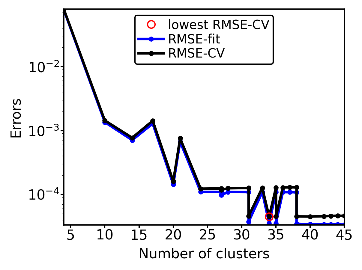
Visualizing results
Last, we visualize model optimization. In the following plot, we can see the RSME fit and CV errors as a function of the number of clusters. We generate an log scale plot, because the resulting errors span several orders of magnitude.
[21]:
plot_optimization_vs_number_of_clusters(mb.get_selector(),
                                        scale=0.7,
                                        show_plot=False)
plt.yscale("log")
plt.show()
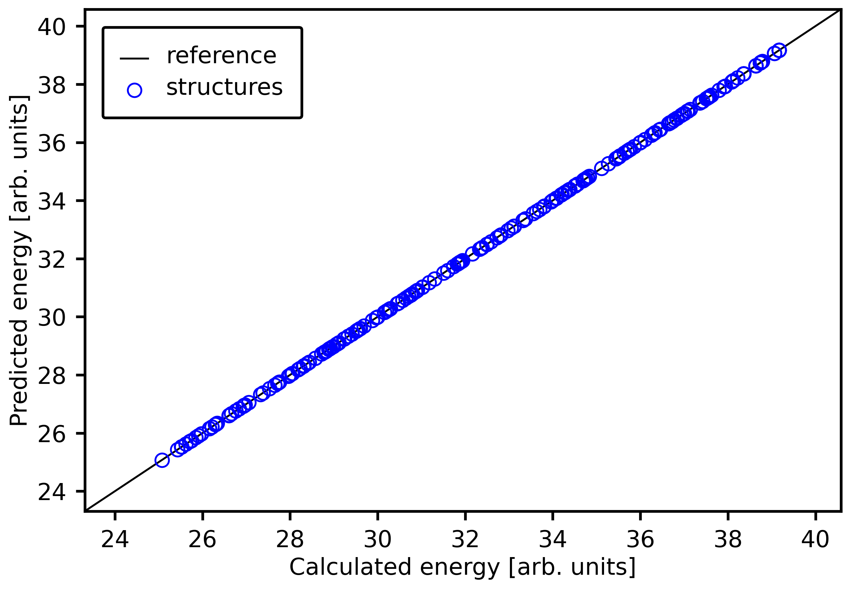
We can show a parity plot to show how the true and predicted energies relate to each other:
[23]:
plot_predictions_vs_target(alloy_dot_sset,
                           cemodel,
                           "total_energy",
                           scale=0.7)
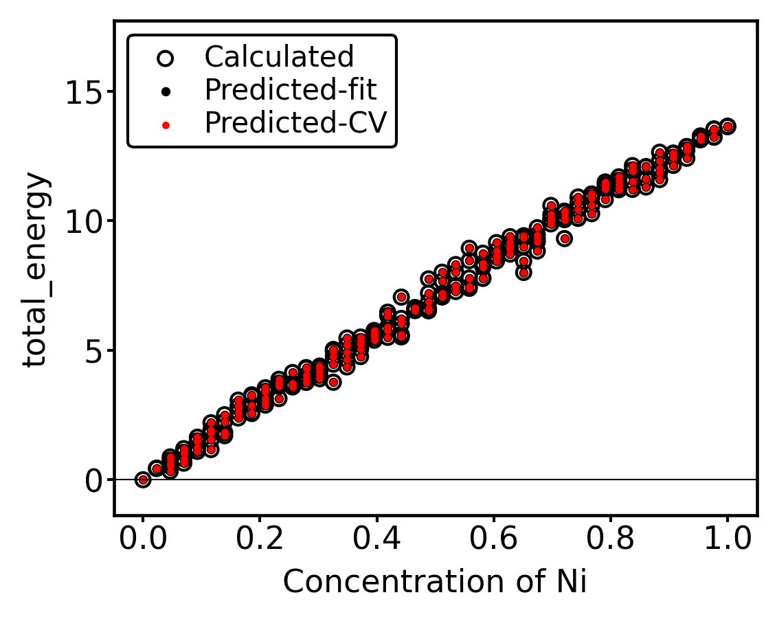
Lastly, the property vs concentration plot shows us that the quality of predictions is high over the full configuration range:
[24]:
_ = plot_property_vs_concentration(alloy_dot_sset,
                               site_type=0,
                               property_name="total_energy",
                               cemodel=cemodel,
                               refs=energies,
                               scale=0.7)